Host software

Everything that runs on the PC: the viewer, the recorder, and the naneye Python package they are built on, for your own scripts. It is Python, managed with uv, and lives in host/naneye. First time? Start with Getting started.

uv sync                  # from uv.lock
uv sync --extra saleae   # adds logic2-automation
uv sync --group docs     # adds mkdocs-material

The sources abstraction

Every tool takes a --source, and all of them accept the same kinds. This is the reason the host side could be built and tested before any hardware existed: replay re-encodes reference frames through the real wire protocol, so what a tool receives is byte-for-byte what the Teensy would send.

--source	What it is
replay	reference frames from build/golden, or generated ones if that is absent
auto	the first Teensy serial port found (PJRC VID 0x16C0 preferred)
COM7	that serial port
a .csv path	a Saleae capture of the link, decoded and played back as frames
a file path	a recorded packet stream

uv run python -m naneye.viewer --source doc/digital.csv

Pointing it at a capture decodes the raw logic-analyser export: bits sampled on SCLK rising edges, rows found by the training-pattern alternation break, and each frame re-encoded through the wire format so the viewer sees what it would see from the device. The clock rate comes from the capture's own edge timing, so exposure and SCLK in the status bar are measured rather than assumed, and per-frame start/stop-bit failures land in rows_failed.

Sampling a 434 MB export takes ~50 s, so the bit stream is cached under build/golden with a source.json recording which capture produced it. An unlabelled cache is spot-checked against the first 20,000 edges rather than trusted blindly.

replay no longer requires the reference capture: without it you get generated frames, labelled SYNTHETIC in the source name so they cannot be mistaken for sensor data.

from naneye.sources import open_source

with open_source("replay", fps=19.3) as src:
    for header, img in src.frames():
        print(header.describe(), img.shape, img.dtype)

Camera GUI

The main way to look at the camera: a PyQt6 application.

uv run python -m naneye.gui                                   # live camera, 49.5 MHz
uv run python -m naneye.gui --source replay                   # no camera needed
uv run python -m naneye.gui --snapshot gui.png                # screenshot after 4 s, then exit

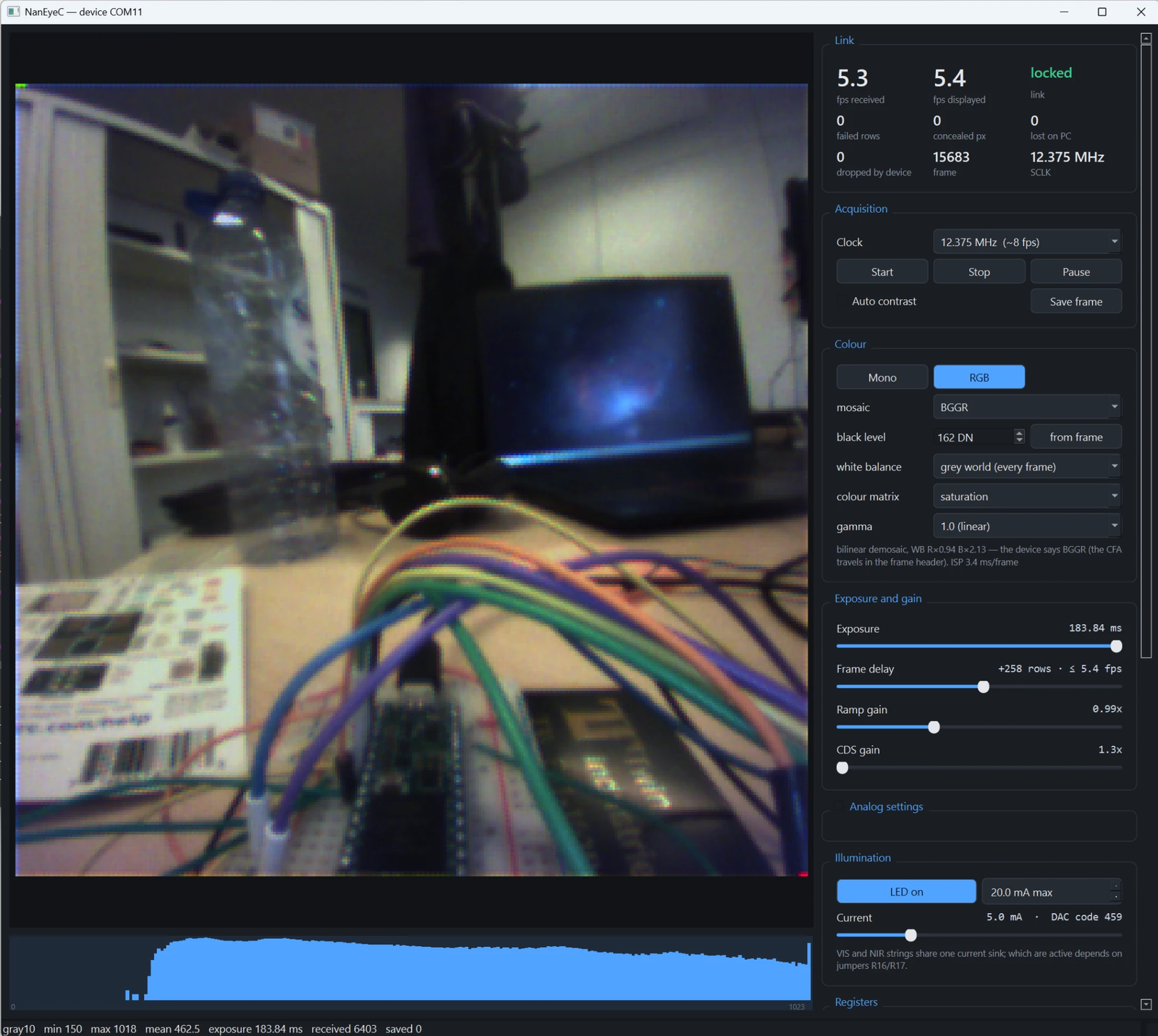
Streaming from a colour sensor at 12.375 MHz. Everything below the image is described in the table.

Panel	What it shows
Link	fps received: frames that arrived over USB intact, per second. fps displayed: frames painted. Link lock state, failed rows, concealed px, lost on PC (left the device, never arrived intact), dropped by device (skipped by the firmware because the PC had not taken the previous frame yet), frame counter, SCLK
Acquisition	Clock rate, Start, Stop, Pause, auto contrast, Save frame (16-bit PNG, raw values). Start powers the sensor and streams; Stop powers it off
Exposure and gain	Sliders for exposure, frame delay, ramp gain and CDS gain, each read out in real units (ms, fps, ×)
Colour	The Mono / RGB switch, the mosaic, and the ISP: black level, white balance, colour matrix, gamma, highlight repair. The caption says what the device reported and how long the ISP took
Detail	Interpolation, denoise and sharpening: the three that trade time for looks, each selectable and each measured in the table below
Analog settings	Sliders for the six analog fields, amber when not at the datasheet's recommended value, and a Datasheet recommended button. Collapsible
Illumination	The NanoBerry's LEDs: on/off, current in 0.1 mA steps with the DAC code it becomes, and the current ceiling (LEDMAX, default 20 mA, hardware maximum 44.6 mA). Switching on sends the current first, because the DAC powers up at zero
Registers	Both registers decoded field by field; firmware-owned fields grey
Device	Every command sent and every reply, including START's sampling-point report

Under the image is a log-scaled histogram of the raw 10-bit values, with the display window shaded: the two raw values that land on 0 and on 255 on screen. Its low end is the black level, or the auto-contrast floor when that is higher; its high end is full scale, or the auto-contrast ceiling. Everything outside the shading is clipped, and the shading is the only honest way to see that.

It used to lie, and the lie was invisible

The window was measured on the ISP's output — after the black level and the white balance — and then drawn against an axis of raw values. With a black level of 170 DN and a blue gain of 1.4, the shading sat a couple of hundred DN to the left of the pixels it claimed to describe. Worse, the auto-contrast percentiles were taken with a stride of 2 over the mosaic, which lands on a single Bayer site: on the colour sensor the automatic contrast was set by the blue pixels alone. Both are fixed; the window is now decided on the raw mosaic, over all four sites, and the pipeline is told to honour it.

Green passes through white balance at gain 1.0, so a green pixel at the top of the window comes out at exactly 255. Red and blue land wherever their gains put them, and with the saturation matrix on, a green pixel reaches 246 rather than 255 because the matrix mixes a little red and blue back out of it. That is the matrix working, not the window slipping.

The whole side panel, top to bottom. In the window it scrolls.

Key	Action
+ / -	longer / shorter exposure
R	datasheet-recommended analog settings
L	LED on/off
[ / ]	LED current ∓1 mA
S	save the frame (16-bit PNG, raw 10-bit values)
Space	pause
Q	quit

The panels only ever show the device's own state or what was sent to it: the register table and the Link panel come from each frame's header, and every command and reply is in the Device log. The LED settings are the exception, because frames do not carry them; the GUI sends its LED state to the device when it starts, so the two cannot disagree.

How it keeps up. A background thread owns the serial port and reads every packet as it arrives; the window paints the newest frame at up to 60 Hz. So a slow repaint skips frames on screen only, never in reception. The two fps figures make that visible, and the frame accounting makes loss visible: a gap in the frame counter that the device's header accounts for is dropped by device, anything else is lost on PC. Measured at 49.5 MHz: 35.5 fps received, 35.5 displayed, nothing lost or dropped over 45 s.

Commands are only ever written from the window (Device.command()); their replies arrive in the packet stream and are picked up by the reader thread. Nothing competes for the port.

Recovery. If the serial port fails, because the Teensy was unplugged or its watchdog reset it, the link shows RECONNECTING. The reader closes the port and tries every second to open it again, first under its old name, then any Teensy. Once it is back, the camera is restarted and the slider and LED settings are written back, since a reset device comes back with its defaults. If the port is fine but frames stop, the link shows NO FRAMES after 2 s, and after 5 s the camera is restarted, unless Stop was pressed. Everything is logged in the Device panel. The device is started only once the window and its reader are running: started earlier, it streamed while the window was being built and dropped frames nobody was reading (124 of them, in the measurement that found this).

Power follows the window. Opening the GUI powers the sensor and starts it; Stop sends STOP then POWER 0, and closing the window sends STOP, LED 0 and POWER 0 before it lets go of the port. So a closed GUI leaves the bench dark, unclocked and with the sensor's rail down, and Start brings it all back — START power-cycles the sensor anyway. The same is true of any DeviceSource, the recorder included: closing one powers the board down.

Colour, and the ISP

A colour NanEyeC has a Bayer filter over the pixels and streams the mosaic exactly as a mono one streams pixels: nothing in the data says which is which. So the firmware is told once — CFA BGGR, kept in EEPROM — and it repeats the answer in the flags of every frame header. The GUI follows that automatically and a recording is still readable years later. The datasheet (6.3.1) fixes the pattern: the first pixel read out is the bottom-left one and is blue, which makes the array as received BGGR.

The Mono / RGB switch decides what you look at. Mono shows the raw mosaic as it arrives, which is what you want when measuring; RGB runs the ISP. The switch follows the device until you touch it, after which it is yours. C toggles it.

What the camera comes up as

The defaults are the ones that suit the colour sensor on this bench, and they live in one dictionary, gui.DEFAULTS:

		Why
Clock	12.375 MHz	the slowest of the three, and so the longest exposure the sensor allows
Exposure	maximum (rows_in_reset = 0)	the colour part sees little light; sent once, on the first frame that says where the registers are, and never again
Auto contrast	off	the ISP has a black level and a tone curve now, and a stretch on top of them fights both
Mode	RGB, BGGR	still switchable, and still overridden by a device that reports mono
Black level	170 DN	measured on this sensor, not a datasheet figure
White balance	grey world, every frame
Colour matrix	saturation	uncalibrated, and the picture looks right
Gamma	sRGB

Every one of them is a control in the window; this is only where they start. --clock overrides the first.

The pipeline

black level  ->  white balance  ->  demosaic  ->  colour matrix  ->  gamma

black level -> white balance -> demosaic -> highlight repair -> colour matrix
            -> denoise -> sharpen -> gamma

Stage	Choices	Why it is that cheap
Black level	a pedestal in DN	a constant; folded into the white balance multiply
White balance	off, grey world once, grey world every frame	applied on the mosaic, where there is a quarter of the data, as one multiply by a precomputed gain map
Demosaic	bilinear or gradient corrected	bilinear is separable [1,2,1] kernels with the weights precomputed; gradient corrected (Malvar-He-Cutler) adds a few fixed taps and no decisions per pixel
Highlight repair	leave, clip to white, reconstruct	decided per channel; everything after the test works on the list of damaged pixels, so it follows the damage rather than the frame
Colour matrix	none, saturation, calibrated	a single matmul, which NumPy gives to BLAS
Denoise	off, colour noise, colour and luma	chroma is smooth where luma is not, so two box passes over three chroma planes cost little and soften nothing
Sharpen	off, light, medium, strong	unsharp mask on luma only: one box pass and an add
Gamma	2.2, 1.8, linear or sRGB	a 1024-entry lookup table: an array index, not a power per pixel

Bold is the default. Measured on a real frame from this sensor, 320 × 320, median of 30:

	ms a frame
bare pipeline (bilinear, nothing else)	2.5
+ gradient-corrected interpolation	+4.2
+ highlight reconstruction	+1.9
+ colour denoise	+1.1
+ colour and luma denoise	+3.3
+ sharpen	+0.4
the defaults	9.8
everything at maximum	12.2

The budget is 20 ms a frame. What the choices buy, measured live on the sensor by two proxies — colour changing at the Bayer pitch, which no scene can do and only a demosaic artefact does, and mean luma gradient, which is detail:

	colour artefacts	detail
bilinear, nothing else	4.97	3.71
gradient corrected	3.32	5.07
bilinear + colour denoise	1.05	3.94
the defaults	1.23	5.84

Four times fewer colour artefacts and 57 % more detail than plain bilinear, for 4 ms.

Speed is the point, not fidelity — this is the viewfinder of a measurement camera, and the thing that gets recorded and measured is the raw 10-bit mosaic. Measured on the bench at 320 × 320: 2.3 ms a frame with every stage on, 1.6 ms without the colour matrix, 0.3 ms in mono. A frame at 35 fps allows 28 ms. The GUI shows the live figure in the Colour panel's caption, so it cannot quietly rot.

Not included, deliberately: lens shading, denoise, sharpening, defect correction, local tone mapping. None of them would make a measurement truer, and all of them invent data.

Why blown highlights came out pink

The sensor clips every channel at the same raw value. White balance then multiplies them by different gains, each clips separately at the white point, and what was equal is not equal any more. With the gains this bench measures — R ×1.11, B ×1.44 — a neutral pixel at the ceiling arrives as R 947, G 853, B 1023, and the saturation matrix finishes the job at R 963, G 792, B 1023. That is pink, and no amount of tuning further down the pipeline can undo it: the information that all three channels were equal is gone by then.

So it is caught where it still exists. Before anything scales the channels apart, pixels at or above SATURATED (1015 DN, against a measured sensor ceiling of 1018–1022) are marked on the mosaic; after the colour matrix, those pixels are set to white. The mask is spread through the same 3×3 support the demosaic uses, because one clipped site bleeds into every neighbour it is interpolated into.

Measured on recorded frames from this sensor: blown pixels averaged R 235, G 229, B 255 before, and R 255, G 255, B 255 after. The Colour panel's blown highlights to white switch turns it off, for anyone who would rather see where the clipping is than have it rendered politely.

What is honest and what is not

Measured	the mosaic phase: the two green sites are the (0,1)/(1,0) diagonal, by sub-lattice correlation (0.64 against 0.43) and by their response to the board's white LED (+56 DN against +40 DN)
From the datasheet	that the (0,0) corner is blue and not red. Nothing in a frame can tell red from blue, and the white LED lifts both corners equally, so this one is on the datasheet's word. If your reds and blues are swapped, the mosaic list in the panel is one click away
Not calibrated	the colour matrix. none is the default and is the honest one; saturation is a mild lift that makes the preview look like a camera and says nothing true about colour. A real matrix comes from a colour chart, which this project has not shot
Not calibrated	the black level. from frame takes the darkest 1 % of what is in view, which beats zero and is not a dark frame

From Python, without the GUI:

from naneye.isp import Isp
from naneye.sources import open_source

isp = Isp(pattern="BGGR", black_level=64, gamma=2.2)
with open_source("auto") as src:
    for header, raw in src.frames():
        isp.pattern = header.cfa          # the frame says what it is
        rgb8 = isp.process(raw)           # (320, 320, 3) uint8
        linear = isp.linear(raw)          # float32, pre-gamma, for measurement

Lightweight viewer

The original OpenCV viewer is still there. It has fewer controls, and at 35 fps it cannot always keep up, but it needs no Qt.

uv run python -m naneye.viewer --source auto                           # live camera, 49.5 MHz
uv run python -m naneye.viewer --source replay                         # no camera needed
uv run python -m naneye.viewer --source auto --snapshot shot.png       # one frame, no window

--depth selects 10-bit (default) or 12 (raw pixel periods, a diagnostic format).

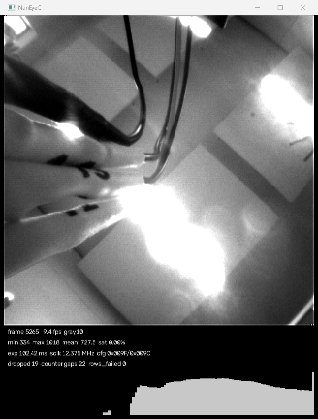
The status bar is the point of it: frame counter and rate, min/max/mean, saturated percentage, exposure in ms, SCLK, both config registers, and the numbers that tell you whether to trust the data: dropped, counter gaps, rows_failed and concealed. SYNC LOST turns red.

Register panel

Beside the image, both sensor registers are decoded field by field, with each value's meaning in real units: exposure in ms, the frame-rate ceiling, gains, voltages, drive current. Fields marked * are not at the datasheet's recommended value. Grey fields marked (fw) belong to the firmware (output mode, idle, and the clock bits that must match SCLK) and cannot be changed from the viewer. G hides the panel.

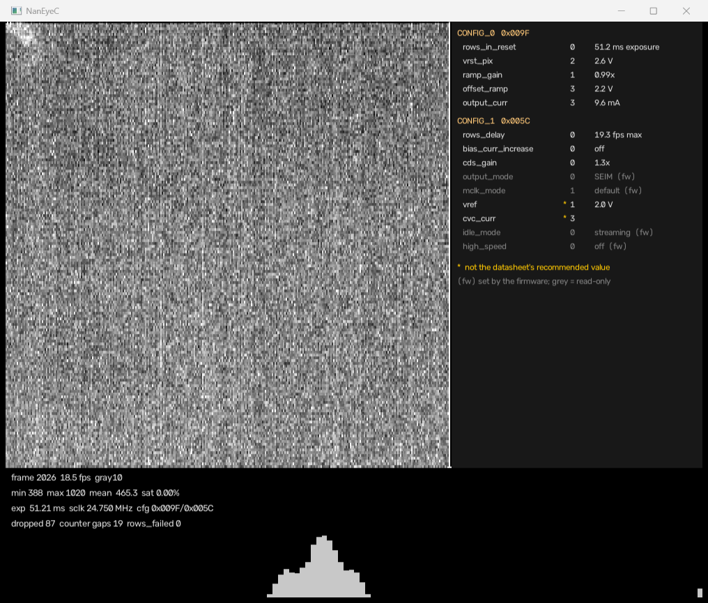
Here the camera was looking at something dark, so auto-contrast stretches a ~40 DN range into noise.

Controls

With a live camera, a second window, NanEyeC controls, has a slider for every field that is safe to change while streaming. Below the sliders is what each one means, and whether it is already in force on the sensor or still sending.

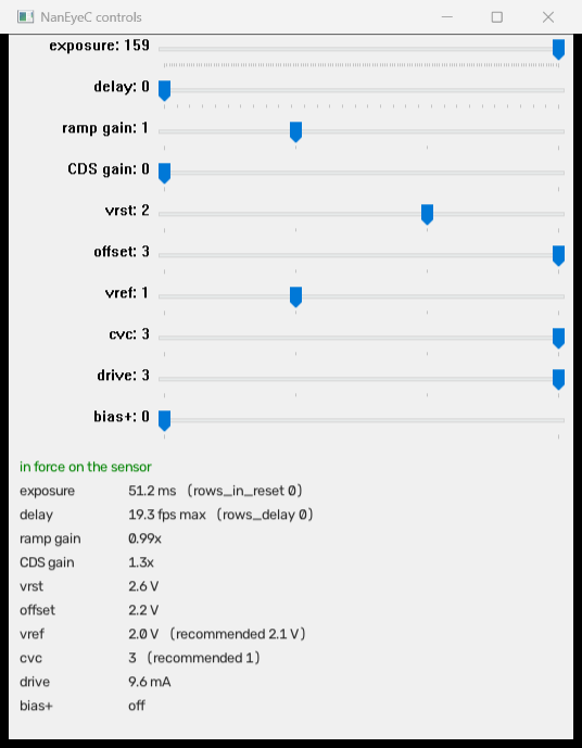
Slider	Field	What it does
exposure	rows_in_reset	right = longer. 1.3–102 ms at 12.375 MHz, half that at 24.75 MHz
delay	rows_delay	adds 16n + 2 rows per frame: slower frame rate, longer maximum exposure
ramp gain	ramp_gain	ADC gain 0.79× / 0.99× / 1.32× / 1.97×
CDS gain	cds_gain	column amplifier 1.3× / 2.0×
vrst	vrst_pix	pixel reset voltage
offset	offset_ramp	ADC ramp offset voltage
vref	vref	ADC reference; sets the black level
cvc	cvc_curr	column converter current; affects column noise
drive	output_curr	SDAT output drive, 3.9–9.6 mA; lower is quieter but gives slower edges
bias+	bias_curr_increase	pixel bias current

A change is sent once the slider has been still for 0.15 s, as a write of the whole register, and takes effect on the next frame. The device stays the source of truth: the sliders start from the registers in the first frame, and the firmware-owned bits are always taken from the latest frame. All of this was checked on hardware, including frame delays up to 31, with no failed rows.

Recommended is not automatically better

D sets the datasheet's recommended analog values. On the same dark scene at 24.75 MHz, vref 1 → 2 lowered the black level by 76–130 DN (more usable range), but cvc_curr 3 → 1 doubled the column fixed-pattern noise (4.3 → 8.4 DN). vref = 2 with cvc_curr = 3 measured best. That is one scene and one clock rate, not a characterisation.

Key	Action
Q / Esc	quit
S	save the current frame as PNG
R	raw vs autoscaled contrast
H	histogram on/off
G	register panel on/off
D	datasheet-recommended analog settings (moves the sliders)
Space	pause
+ / -	longer / shorter exposure (moves the exposure slider)
L	LED on/off
[ / ]	LED current ∓1 mA

The register model behind all this is naneye.regs: every field with its position, units, recommended value and whether it is safe to edit, plus the exposure and frame-period maths.

from naneye import regs
print("
".join(regs.describe(0x009F, 0x005C, sclk_hz=24.75e6)))
c0, c1 = regs.pack({"ramp_gain": 2, "rows_delay": 4}, 0x009F, 0x005C)

--snapshot composes exactly what the window shows and writes it to a file: handy for bug reports and for documenting a setup. The viewer holds the serial port while it is open, so close it before running a script or the recorder.

Recorder

uv run python -m naneye.record --source auto --frames 1200 --out capture/run1
uv run python -m naneye.record --source auto --seconds 60 --exposure 64 --out capture/run2
uv run python -m naneye.record --source auto --seconds 600 --no-frames --out capture/soak

Per run:

File	Contents
frames.npy	(N, 320, 320), uint16
meta.csv	one row per frame: counter, timestamp, exposure, config, drop counters, failed rows, concealed pixels, min/max/mean
run.json	settings and a summary: measured fps, frames dropped by device and lost on PC (kept apart, as in the GUI), failed rows, concealed pixels, and packets the host rejected (host_bad_crc, host_resyncs)
stream.bin	with --raw, every packet header

Frames go to disk as they arrive, so memory stays flat however long the run. They are written to frames.bin and meta.csv is flushed as it goes, so if the recorder dies, everything received so far is still there: np.fromfile("frames.bin", np.uint16).reshape(-1, 320, 320). At the end frames.bin is copied into frames.npy in chunks and removed (--keep-bin keeps it). Mind the disk: at 49.5 MHz, 10-bit data is about 7 MB/s, so a 10-minute run is about 4.3 GB, and briefly twice that while frames.npy is assembled.

--no-frames writes only meta.csv and run.json: every frame's header and statistics, no pixels. That is what a soak test of the link needs.

For a live device the recorder starts the camera itself, once it is already reading, and ignores anything from an earlier stream until START has answered, so no frames pile up unread at the start. --seconds times the run instead of counting frames.

A recording is self-describing: every frame carried its own exposure, gain, clock rate and drop counters in its header, so nothing has to be remembered separately. For measurement work that matters more than it sounds — it is what lets you come back to data months later and still know what it is.

import json, numpy as np
frames = np.load("capture/run1/frames.npy")
meta = json.load(open("capture/run1/run.json"))
assert meta["lost_on_pc"] == 0 and meta["dropped_by_device"] == 0
assert meta["rows_failed_total"] == 0
dark = frames.mean(axis=0)
print("temporal noise", frames.astype(float).std(axis=0).mean(), "DN")

Decoding

naneye.decode is the canonical decoder, used for live frames, Saleae captures and the golden-capture tool alike.

from naneye import decode

# Device payloads
img = decode.decode_payload(header, payload)      # -> (320, 320)
img = decode.raw12_to_image(raw)                  # drop per-row training words

# Pixel periods from 32-bit words (mirrors the firmware exactly)
pp = decode.words_to_pp(words, decode.ROW_PP)
ok = decode.validate_pp(pp)                       # start=1, stop=0
px = decode.pp_to_pixels(pp)

# Logic-analyser captures
bits, times = decode.sample_saleae_csv("capture.csv")
for i, img, stats in decode.decode_frames_from_bits(bits):
    assert stats["bad_start_bits"] == 0
idx, lens = decode.find_clock_gaps(times, threshold_s=1e-6)
writes = decode.decode_register_writes(bits[:200])

decode_frames_from_bits finds rows by the alternation break and yields only frames whose row pitch is exactly 3936 bits, so a malformed capture is skipped rather than silently mis-decoded.

Protocol

naneye.protocol mirrors firmware/src/usb_proto.h. A 52-byte little-endian header, CRC-32 over header bytes 0–47 plus the payload, then the payload.

from naneye import protocol
h = protocol.Header.unpack(buf)
print(h.describe(), h.exposure_us(), h.sync_lost)

transport.PacketReader resynchronises on the magic word and verifies every CRC, so a corrupted or partial packet costs one frame rather than the stream. It works over any read(n) callable — serial port, socket, file, BytesIO — which is what makes it testable.

from naneye.transport import Device
with Device.open_first() as dev:
    print(dev.ask("ID"))
    print(dev.ask("SELFTEST"))
    dev.command("START")
    for pkt in dev.frames():
        ...

Commands

The firmware takes plain text lines; replies come back framed, so use Device.ask() rather than a serial terminal. Commands are processed between frames, so a reply can take up to one frame period to arrive while streaming.

Command	What it does
ID	firmware version, actual SCLK, registers, format, last reset cause
CLK 49500000	SCLK rate: 49500000 (~35 fps), 24750000 (~18 fps) or 12375000 (~8 fps). The host tools default to 49.5 MHz
START	power-cycle the sensor, start it, choose the sampling point, lock onto its rows, check 8 rows, stream (takes ~1.2 s). The reply reports what the calibration measured
STOP	stop streaming (the sensor stays powered, in idle)
POWER 0 / POWER 1	sensor power; switching on waits until it has been off ≥ 1 s
DEPTH 10 / 12	packed 10-bit (default), or raw 12-bit pixel periods (diagnostic)
EXP <rows_in_reset> [rows_delay]	exposure: 0 longest (~102 ms at 12.375 MHz) … 159 shortest (~1.3 ms); rows_delay slows the frame rate
REG <reg> <0xHHHH> (reg 0 or 1)	raw register write, validated
LED 0 / LED 1, LEDI <mA>, LEDMAX <mA>	illumination: on/off, current (clamped, default ceiling 20 mA), raise the clamp up to 44.6 mA. LED 1 alone gives almost no light; set LEDI first
STATS	frame counters and link state
SELFTEST	check decoding and exposure maths against the embedded reference row

Diagnostic commands (LISTEN, PROBE, START REF, CAL, SAMPLE, PHASE, HYS) are described in Firmware: diagnostics.

Tests

uv run pytest          # 112 tests, none needing hardware

File	Covers
test_protocol.py	every header field offset against the firmware's static_asserts, CRC behaviour
test_unpack.py	pixel extraction against the golden row, lossless 10-bit packing
test_transport.py	CRC rejection, resync past junk, truncation, drop accounting
test_golden.py	the reference capture: row pitch, start/stop bits, noise, mono, registers, the gap defect
test_sources.py	replay path resolution, the synthetic fallback, lossless replay round-trip
test_device.py	the Device command/reply logic against a simulated serial port
test_regs.py	the register model: field layout, round trips, exposure maths against the firmware and the device
test_gui.py	the Qt GUI, headless: loss accounting (device drops vs PC losses), frame hand-over, reconnecting after the port fails, and a smoke test on replayed frames
test_record.py	the streaming recorder end to end: frames.npy against meta.csv, the raw stream, --no-frames, the raw 12-bit format
test_link_quality.py	the link-quality analysis: alignment search, framing-error counting, and the limit that data-bit errors are invisible

Tests needing the 434 MB capture skip cleanly when it is absent. test_unpack.py parses the generated golden_vector.h so the Python decoder is held to the exact data the device's SELFTEST checks itself against — the C and Python implementations cannot diverge silently.

Tools

uv run python tools/decode_golden.py [capture.csv] [--out build/golden]
uv run python tools/make_golden_vector.py --row 200

decode_golden.py is the reference decode and the regression baseline: it reports clock rate, register writes with fields expanded, per-frame validation, temporal noise and the mono check. It caches bits.npy, so only the first parse costs ~50 s.

make_golden_vector.py regenerates the firmware's embedded test row. Pick a clean row — rows 129 and 262 of the reference frame 1 contain the host's clock-gap corruption.

With a Saleae logic analyser and its Logic 2 software running (MCP server enabled), these capture the live link and analyse it; host/naneye/saleae.py is the client they share:

Tool	What it does
tools/device_check.py	ID, SELFTEST and STATS; no analyser needed
tools/link_quality.py	word error rate at every sampling point, at a given clock; no analyser needed
tools/show_bringup.py	triggers on sensor power-up, runs a start command and plots what happened
tools/check_alignment.py	shows where each row transfer lands relative to the sensor's rows
tools/capture_link.py, tools/analyze_link.py	general captures: clock rate, phase counts, register writes